
Imagine you’re trying to predict which customers are likely to churn. A decision tree can help, but how deep should it be? Too shallow, and it might miss crucial patterns. Too deep, and it might memorise the training data, failing to generalize to new customers.
This post builds on the “Decision-Tree” post and dives into the critical concept of tree depth in decision trees, exploring its impact on model performance and providing practical techniques to optimise it.
Let’s keep the following definitions in mind as we build our understanding:
- Tree Depth: The number of levels in a decision tree from root to the deepest leaf node.
- Overfitting: When a model learns patterns too specific to the training data, reducing generalisation.
- Underfitting: When a model is too simple and fails to capture the patterns in data.
- Pruning: The process of removing unnecessary branches from a decision tree to prevent overfitting.
- max_depth: A parameter that limits the maximum depth of a decision tree.
- min_samples_split: The minimum number of samples required to split an internal node.
- min_samples_leaf: The minimum number of samples that must be present in a leaf node.
- ccp_alpha: A parameter for cost complexity pruning, controlling how aggressively a tree is pruned.
The depth of a tree determines how complex the model is, influencing both accuracy and generalisation. In this follow-up blog, we will explore:
- What tree depth means in Decision Trees
- The impact of tree depth on model performance
- Practical ways to control and optimise tree depth
What is Tree Depth in Decision Trees?
Tree depth refers to the number of levels in a decision tree, from the root node to the deepest leaf node. It plays a crucial role in how well the tree can model patterns in data.
- Shallow Trees (Low Depth): Capture only basic patterns. Think of it as a simple “if-then” rule. They are less prone to overfitting but may underfit the data, leading to lower accuracy.
- Deep Trees (High Depth): Capture intricate patterns, potentially revealing complex relationships. However, they are highly susceptible to overfitting, performing well on training data but poorly on unseen data.

Impact of Tree Depth on Model Performance
The table below outlines how different aspects of model performance are influenced by tree depth:
| Aspect | Effect of Low Depth (Shallow Trees) | Effect of High Depth (Deep Trees) |
|---|---|---|
| Accuracy | Lower accuracy, may underfit data | High training accuracy, may overfit |
| Generalization | Better generalization to new data | Poor generalization, risk of overfitting |
| Computational Cost | Lower, faster training & inference | Higher, increased computation time |
| Interpretability | Easier to understand and visualize | Complex and difficult to interpret |
Problems Caused by Unchecked Tree Depth
When tree depth is not controlled, several issues can arise:
- Severe Overfitting
- Deep trees memorize training data rather than generalizing patterns.
- High training accuracy but poor test performance.
- Increased Computational Costs
- Larger trees require more storage and processing power.
- Training and inference times increase significantly.
- Decreased Interpretability
- Complex trees become difficult for humans to interpret and analyze.
- Hard to extract meaningful decision rules from deep trees.
Controlling Tree Depth: Pruning and Hyperparameter Tuning
Pruning is a crucial technique for preventing overfitting. It involves removing branches that contribute little to the model’s accuracy, simplifying the tree and improving generalization.
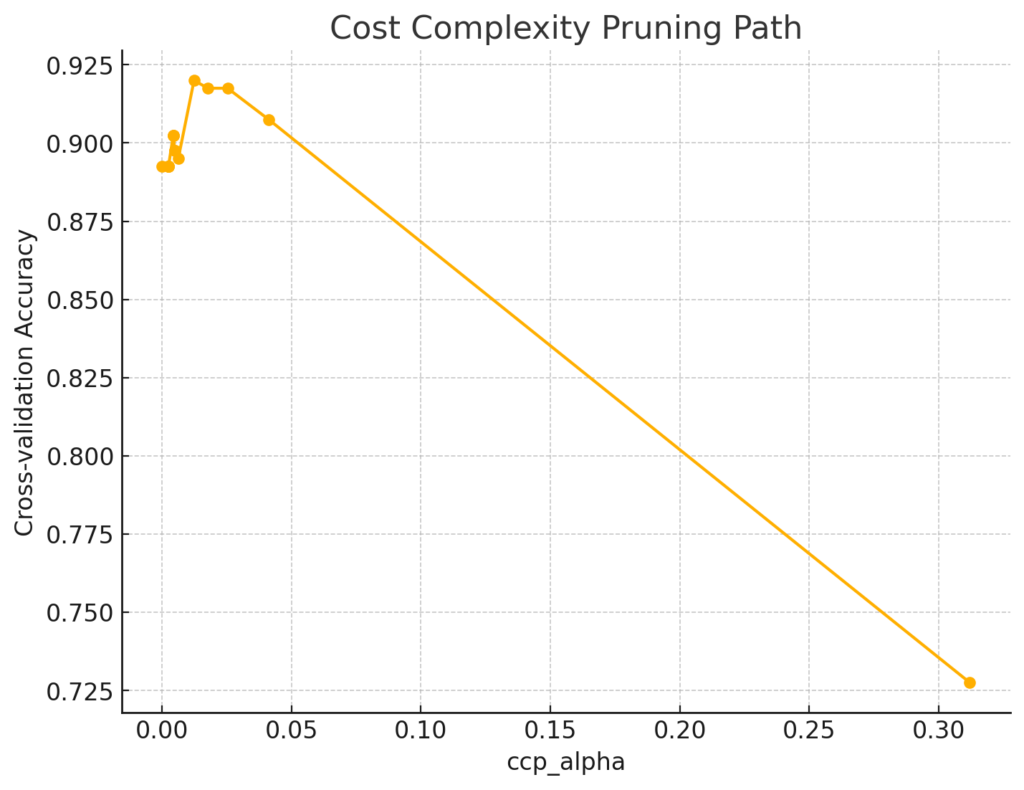
One common pruning method is cost complexity pruning. This method introduces a parameter, ccp_alpha, which controls how aggressively the tree is pruned. A higher ccp_alpha value leads to more aggressive pruning, resulting in a smaller tree. Conversely, a lower ccp_alpha value results in less pruning and a larger tree.
Sample code to show the usage:
# Import necessary libraries
import numpy as np
import matplotlib.pyplot as plt
from sklearn.tree import DecisionTreeClassifier
from sklearn.model_selection import train_test_split, cross_val_score
# Generate sample data
X, y = make_classification(n_samples=500, n_features=10, random_state=42)
X_train, X_test, y_train, y_test = train_test_split(X, y, test_size=0.2, random_state=42)

# Initialize a Decision Tree classifier
clf = DecisionTreeClassifier(random_state=0)
path = clf.cost_complexity_pruning_path(X_train, y_train)
ccp_alphas = path.ccp_alphas

# Find the best ccp_alpha using cross-validation
clfs = []
for ccp_alpha in ccp_alphas:
    clf = DecisionTreeClassifier(ccp_alpha=ccp_alpha, random_state=0)
    scores = cross_val_score(clf, X_train, y_train, cv=5)  # 5-fold cross-validation
    clfs.append((clf, scores.mean()))  # Store the classifier and its mean score

# Select the best classifier based on highest cross-validation accuracy
best_clf, best_score = max(clfs, key=lambda item: item[1])

# Train the best-pruned tree
clf_pruned = DecisionTreeClassifier(ccp_alpha=best_clf.ccp_alpha, random_state=0)
clf_pruned.fit(X_train, y_train)

# Plotting ccp_alpha vs accuracy
scores = [score for _, score in clfs]
plt.figure(figsize=(8, 6))
plt.plot(ccp_alphas, scores, marker='o', linestyle='-')
plt.xlabel("ccp_alpha")
plt.ylabel("Cross-validation Accuracy")
plt.title("Cost Complexity Pruning Path")
plt.grid(True)
plt.show()

# Evaluate the pruned tree
train_accuracy = clf_pruned.score(X_train, y_train)
test_accuracy = clf_pruned.score(X_test, y_test)

# Print results
print(f"Pruned Tree - Training Accuracy: {train_accuracy:.2f}, Test Accuracy: {test_accuracy:.2f}")
Hyperparameter Tuning: min_samples_split and min_samples_leaf
Besides max_depth and ccp_alpha, other important hyperparameters control tree growth:
min_samples_split: The minimum number of samples required to split an internal node. Increasing this value can prevent the tree from creating very specific branches based on small, potentially noisy subsets of the data. For example,min_samples_split=10would require at least 10 samples to be present in a node before it can be split further.min_samples_leaf: The minimum number of samples required to be at a leaf node. This parameter prevents the creation of leaf nodes with very few samples, which can be prone to overfitting. For instance,min_samples_leaf=5ensures that every leaf node has at least 5 samples.
Tuning these parameters (often in conjunction with max_depth and ccp_alpha using techniques like GridSearchCV or RandomizedSearchCV) is crucial for finding the optimal balance between model complexity and generalization.
Sample code to show the usage:
import numpy as np
import matplotlib.pyplot as plt
from sklearn.tree import DecisionTreeClassifier
from sklearn.model_selection import train_test_split, GridSearchCV
from sklearn.datasets import make_classification

# Generate sample data
X, y = make_classification(n_samples=1000, n_features=20, random_state=42)
X_train, X_test, y_train, y_test = train_test_split(X, y, test_size=0.2, random_state=42)

# Define the parameter grid
param_grid = {
    'max_depth': [None, 10, 20, 30],
    'min_samples_split': [2, 5, 10],
    'min_samples_leaf': [1, 2, 4],
    'ccp_alpha': np.linspace(0, 0.02, 10)
}

# Initialize the DecisionTreeClassifier
dt = DecisionTreeClassifier(random_state=42)

# Perform GridSearchCV
grid_search = GridSearchCV(dt, param_grid, cv=5, scoring='accuracy')
grid_search.fit(X_train, y_train)

# Print the best hyperparameters and accuracy
print("Best hyperparameters:", grid_search.best_params_)
print("Best cross-validation accuracy:", grid_search.best_score_)

# Train a model with the best hyperparameters
best_dt = grid_search.best_estimator_
best_dt.fit(X_train, y_train)

# Print the tree depth
print("Tree depth:", best_dt.tree_.max_depth)
This results in Best hyperparameters: {'ccp_alpha': 0.006666666666666666, 'max_depth': None, 'min_samples_leaf': 4, 'min_samples_split': 10}
Best cross-validation accuracy: 0.9012499999999999
Tree depth: 4Striking the Right Balance: A Practical Approach
Finding the optimal tree depth involves a combination of experimentation and monitoring. Here’s a suggested approach:
- Start with a reasonable range: Begin by experimenting with a range of max_depth values (e.g., from 3 to 10) and ccp_alpha values (using cost_complexity_pruning_path).
- Use cross-validation: Evaluate the performance of the tree for each combination of hyperparameters using cross-validation.
- Visualize: Plot the cross-validation scores against the hyperparameter values (like the ccp_alpha plot above). This can help you identify trends and find the optimal values.
- Tune other hyperparameters: Optimize min_samples_split and min_samples_leaf using similar techniques.
- Monitor: Continuously monitor the model’s performance on new data and retune the hyperparameters as needed.
Monitoring and Alerting Mechanisms for Tree Depth
To ensure the optimal depth, implementing monitoring and feedback mechanisms can help:
1. Cross-Validation Metrics
Regularly measure performance using cross-validation to detect overfitting or underfitting.
from sklearn.model_selection import cross_val_score
scores = cross_val_score(clf, X_train, y_train, cv=5)
print("Cross-validation accuracy:", scores.mean())
2. Tracking Performance on Validation Data
Compare training and validation accuracy to identify overfitting.
train_accuracy = clf.score(X_train, y_train)
test_accuracy = clf.score(X_test, y_test)
print(f"Training Accuracy: {train_accuracy:.2f}, Test Accuracy: {test_accuracy:.2f}")
3. Feature Importance Analysis
Check which features are influencing predictions and ensure meaningful splits are occurring.
import pandas as pd
feature_importances = pd.Series(clf.feature_importances_, index=feature_names)
print(feature_importances.sort_values(ascending=False))
4. Automated Alerts for Depth Thresholds
Set depth limits and raise warnings if exceeded.
if clf.get_depth() > 10:
    print("Warning: Tree depth exceeds recommended limit!")
Conclusion
Optimising tree depth is essential for building robust and reliable decision tree models. By understanding the impact of tree depth, utilising pruning techniques, and carefully tuning hyperparameters, you can create models that generalise well to unseen data and provide valuable insights. Remember, the goal is not to achieve perfect accuracy on the training data, but to build a model that performs well on new, unseen data.