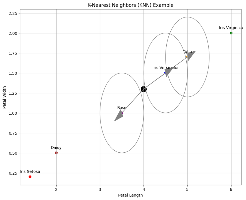
Imagine you have a map with dots representing different types of flowers. If you find a new flower and want to know its type, you could look at the flowers closest to it on the map. If most of the nearby flowers are roses, you might guess that the new flower is also a rose. That’s essentially how KNN works.
How it Works:
- Nearest Neighbor: Finding the closest data points using distances like Euclidean or Manhattan.
- KNN Algorithm:
- Classification: Voting among the ‘K’ closest neighbors.
- Regression: Averaging the values of the ‘K’ closest neighbors.
- Key Points:
- Simple and easy to grasp.
- “Lazy” learning—stores data, doesn’t build complex models.
- Distance matters—choosing the right one is key.
- “K” is crucial—it controls the “neighborhood” size.
Real-World Uses:
- Image & Text Classification: From recognizing faces to sorting emails.
- Predicting Values: Like house prices or stock trends.
- Personalized Recommendations: “If you liked this, you’ll love that!”
- Spotting Oddballs: Detecting fraud or network intrusions.
In a Nutshell:
KNN is like asking your closest friends for advice. It’s intuitive, powerful, and surprisingly versatile!
Let’s Look at Fraud Detection use-case in some detail
Detecting anomalies (outliers) in financial transactions is important for identifying fraud or errors. An anomaly is a transaction that significantly deviates from normal patterns (e.g., an unusually large purchase)
The K-Nearest Neighbors (KNN) algorithm, though typically used for classification/regression, can be adapted for unsupervised anomaly detection by measuring how far each data point is from its neighbors. The intuition is that normal transactions will cluster together, while anomalous transactions will be far away from other points
Approach Overview: Let’s use KNN to compute the distance of each transaction to its nearest neighbors, and flag those with unusually large neighbor distances as anomalies. The steps are:
- Data Preparation: Load a dataset of transactions (or generate a synthetic one) with numeric features (e.g., transaction amount, transaction count).
- KNN Distance Calculation: Apply KNN (unsupervised) to find each point’s nearest neighbors and compute distance metrics.
- Anomaly Identification: Determine a distance threshold (e.g., based on percentile) and label transactions with distances above this threshold as anomalies.
- Visualization: Plot the data points on a scatter plot, highlighting anomalous transactions in a different color for easy identification.
Let’s go through each step with code and explanations.
1. Data Preparation
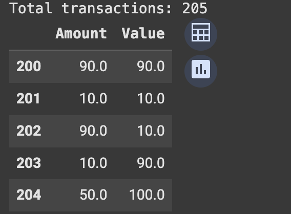
Created num_normal=200 normal transactions with an Amount and Value centered around 50 (using a normal distribution for realism).We then created 5 anomalous points with extreme values (very high or very low compared to 50) to simulate outliers.
# Import necessary libraries
import numpy as np
import pandas as pd
from sklearn.neighbors import NearestNeighbors
import matplotlib.pyplot as plt

# 1. Load or simulate the dataset of financial transactions
# (Here we generate synthetic data for demonstration.)

np.random.seed(42)  # for reproducibility

# Generate a cluster of "normal" transaction data (e.g., Amount and Value around 50 with small variance)
num_normal = 200
normal_amounts = np.random.normal(loc=50, scale=5, size=num_normal)   # e.g., transaction amount around 50
normal_values  = np.random.normal(loc=50, scale=5, size=num_normal)   # another feature (e.g., transaction count or score around 50)
normal_data = pd.DataFrame({
    'Amount': normal_amounts,
    'Value':  normal_values
})

# Generate some "anomalous" transactions that are far from the normal cluster
anomalies = pd.DataFrame({
    'Amount': [90, 10, 90, 10, 50],   # e.g., very high or very low amounts
    'Value':  [90, 10, 10, 90, 100]   # e.g., very high or very low values
})

# Combine normal data and anomalies into one dataset
data = pd.concat([normal_data, anomalies], ignore_index=True)
print(f"Total transactions: {data.shape[0]}")
data.tail(5)  # Show the last 5 transactions (which should be the anomalies we added)
2. Applying KNN to Compute Neighbor Distances
a. extract the feature matrix X from our DataFrame (two columns: Amount and Value).
b. configure NearestNeighbors with n_neighbors=5 (you can adjust K as needed). This means for each transaction, we will look at the 5 closest points (in terms of Euclidean distance by default).
c. after fitting the model on our data, we call kneighbors(X) to get the distances and indices of each point’s 5 nearest neighbors.
d. The result distances is a 2D array where each row corresponds to a transaction, and the 5 columns are the distances to its 1st, 2nd, …, 5th nearest neighbors.
# 2. Use KNN to find distances to nearest neighbors
X = data[['Amount', 'Value']].values  # feature matrix

# Initialize NearestNeighbors model: we'll use k=5 (5 nearest neighbors)
knn = NearestNeighbors(n_neighbors=5)
knn.fit(X)  # fit on the data points

# Compute the distances to the 5 nearest neighbors for each point
distances, indices = knn.kneighbors(X)

# distances is an array of shape (n_samples, 5), where each row contains
# the distances from a point to its 5 nearest neighbors (including itself).
print("Distance array shape:", distances.shape)
print("Example distances for first transaction:", distances[0])

3. Identifying Anomalous Transactions
To flag anomalies, we need to decide on a distance threshold. One common approach is to use a statistical percentile of the neighbor distance measure
For example, we might choose the 95th or 98th percentile of the average distance as the cutoff – meaning we consider the top 5% (or 2%) of points with the largest neighbor distances as anomalies. Here, we will use the average distance to the 5 nearest neighbors for each transaction as an outlier score, and then pick a high percentile as the threshold. Transactions with an average distance above this threshold will be labeled anomalies.
# 3. Determine anomaly threshold based on distances
# Calculate the average distance to the 5 nearest neighbors for each transaction
avg_distances = distances.mean(axis=1)
# Choose a threshold for anomaly (e.g., 98th percentile of the average distances)
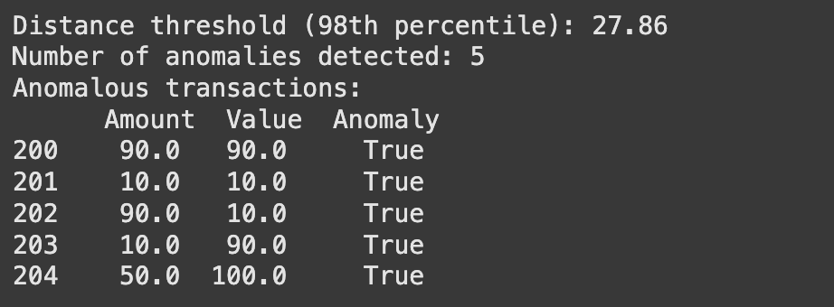
threshold = np.percentile(avg_distances, 98)
print(f"Distance threshold (98th percentile): {threshold:.2f}")
# Flag transactions with average neighbor distance above the threshold as anomalies
anomaly_mask = avg_distances > threshold
data['Anomaly'] = anomaly_mask # add a column indicating anomaly status (True/False)
# Get the indices or count of anomalies for reporting
anomaly_indices = np.where(anomaly_mask)[0]
print(f"Number of anomalies detected: {len(anomaly_indices)}")
# (Optional) Print the anomalous transactions for review
print("Anomalous transactions:\n", data.loc[anomaly_mask])
4. Visualizing the Anomalies
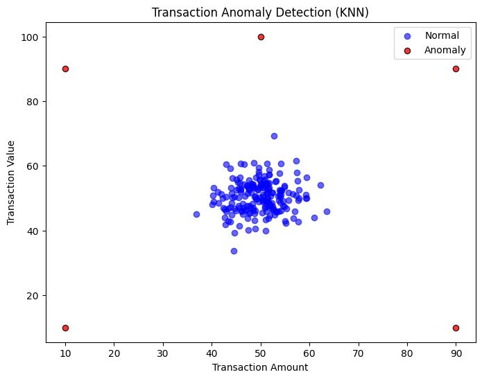
Finally, we will visualize the transactions on a scatter plot to see the separation between normal points and anomalies. We plot the two features on the x and y axes and use different colors or markers for anomalies. In our example, we will plot Amount vs. Value for each transaction, marking normal transactions in blue and anomalies in red. This visual aid helps to verify that the detected outliers are indeed distant from the normal cluster.
# 4. Visualize the anomalies using a scatter plot
# Separate the normal points and anomalies for plotting
normal_data = data[~data['Anomaly']]   # points where Anomaly is False
anomaly_data = data[data['Anomaly']]   # points where Anomaly is True

plt.figure(figsize=(8,6))
# Plot normal transactions in blue
plt.scatter(normal_data['Amount'], normal_data['Value'], c='blue', label='Normal', alpha=0.6)
# Plot anomalous transactions in red
plt.scatter(anomaly_data['Amount'], anomaly_data['Value'], c='red', label='Anomaly', alpha=0.8, edgecolors='k')

plt.title('Transaction Anomaly Detection (KNN)')
plt.xlabel('Transaction Amount')
plt.ylabel('Transaction Value')
plt.legend()
plt.show()
The approach can be adjusted by changing the number of neighbors k or the threshold for flagging anomalies, depending on how strict or lenient you want the detection to be. In practice, you would validate the detected anomalies to ensure they correspond to real issues (such as fraud or errors) and adjust parameters as needed.